Production Jupyter notebooks: A guide to managing dependencies, data, and secrets for reproducibility
It’s one thing to write a once-off Jupyter notebook to do some quick calculations. It’s quite another thing to write a Jupyter notebook for an analytics or machine-learning project that requires iterating on over time, rerunning with new data sets, and collaborating on with your team.
If you write these kinds of notebooks, they need to be reproducible — when the notebook is run at a different time, perhaps on a different machine or by different people, it must run in the same way every time.
In this how-to guide, we’ll offer you some strategies for creating reproducible Jupyter notebooks. Specifically, we’ll cover how to:
- Manage dependencies for your Jupyter notebooks with pip-tools.
- Handle secrets and other environment-specific configurations for your Jupyter notebooks, using environment variables and a
.envfile. - Connect to external data sources in a reproducible way.
1. How to manage dependencies for Jupyter notebooks
Dependency management is the foundation of reproducibility. No one wants to deal with debugging code that has stopped working because of a mysterious change in an underlying dependency. The solution is to ensure that your code is run with the same dependencies each time it is run.
There are a few different patterns for dependency management with Jupyter notebooks.
First, we’ll show you how to pin your Python package dependencies using pip-tools and requirements files. Then we’ll show you how to install these dependencies either directly on your machine using a virtual environment or using Docker.
Pin your dependencies for Jupyter notebooks
Every package used in your project should be explicitly set to ensure that your work is reproducible by future you or your team and in any environment it may be run. Let’s explore a few popular options for managing dependencies in Python.
Conda vs. pip-tools
There are many different options for managing dependencies in the Python ecosystem and all have faced criticism.
One common option is Conda. Conda is a very powerful tool but it can be inflexible and it requires a commercial license for non-personal use.
pip is the default Python package manager and what most Python developers are used to using. pip uses a requirements.txt file to list project dependencies, but requirements.txt files can get large and difficult to manage if you use pip alone. Adding just a single library like Matplotlib can introduce dozens of indirect dependencies to your requirements.txt file.
A good middle ground is pip-tools. pip-tools builds production-level tools on top of pip for the best of both worlds. You’ll maintain a simpler requirements.in file with only direct dependencies, and then use pip-tools to compile this file to the full requirements.txt file.
Here’s a step-by-step guide to getting started with managing your dependencies with pip-tools.
Create a requirements.in file
To start with, gather all the explicit Python dependencies imported in your code in a requirements.in file. It’s generally good practice to order items in your requirements files alphabetically. For example:
# requirements.in

jupyter
numpy
pandas<2
seaborn>=0.11
Note that we specify the versions of some dependencies here: A Seaborn version greater than or equal to 0.11 and a Pandas version less than 2. You can use version conditions if your code needs to use specific versions of dependencies — perhaps you know you need new functionality or you want to avoid a breaking change in a newer version of a dependency.
The requirements.in file gives general instructions for which packages we want. The next step is to turn these general requirements into exact requirements.
Create a requirements.txt file
Our exact requirements will be saved in a requirements.txt file created by the pip-compile command provided by pip-tools. First install pip-tools, then we can compile our requirements:
$ pip install pip-tools
$ pip-compile requirements.in
The pip-compile command chooses the latest compatible version of each package you have specified, subject to the conditions you set in the requirements.in file. It also determines all of the dependencies of the packages you have specified and ensures that the dependency versions are compatible across all of the packages — this is called dependency resolving.
In our example, we only explicitly require four packages but the full package list generated by pip-compile is much longer. Here is the beginning of the generated requirements list:
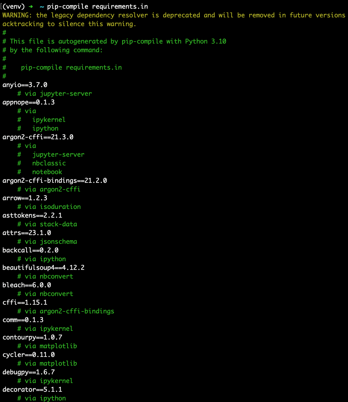
The pip-compile command generates a requirements.txt file containing the full set of dependencies. Note how every package is now pinned at an exact version and the file records which Python version was used to create it. Also note how each dependency is listed with the package it is needed for. For example, countourpy is a dependency of matplotlib and if we scroll further down, we see that matplotlib is a dependency of seaborn.
You should save both the requirements.in and requirements.txt files as part of your project and check them in with your notebooks and code to the version control system you use.
This dependency-pinning step is only necessary when you:
- First set up your project,
- Add new dependencies, or
- Update dependencies.
TIP: If you want to check which Python packages are installed, you can use:
$ pip freeze
If you run this command in a virtual environment, it will list the packages installed in the virtual environment. If you run it outside of a virtual environment, it will list the packages installed on your system.
Install your requirements in a virtual environment
The first option for installing your dependencies is to install them locally in a virtual environment (an isolated environment where you can install Python packages).
First, create a dedicated virtual environment for your project. We’ll use virtualenv. If you haven’t yet installed it, install it from a terminal:
$ pip install virtualenv
Then create a virtualenv for your project. A common pattern is to create it in your project’s Git repository folder and call it venv, then add the folder name venv to a .gitignore file so that the installed dependencies will not be unnecessarily tracked in version control:
$ virtualenv venv
You can specify a Python version here if you want a specific version. It must be a version you already have installed on your machine.
$ virtualenv --python 3.10 venv
Next, activate the virtual environment. You’ll know the virtual environment is active if your prompt now begins with the name of the virtual environment, in our case, venv:
$ source venv/bin/activate
(venv) $
When you’re finished working in the project, you can deactivate the virtual environment to return to your general system Python environment by typing:
> deactivate
But for now, we will continue working in the virtual environment. You only need to create a virtual environment in your project folder once, then you can activate it when you need it and deactivate it when you are finished working on the project.
TIP: If at any point you want a clean virtual environment, you can deactivate the one you have, delete it, and create a new one:
$ deactivate
$ rm -rf venv
$ virtualenv venv
$ source venv/bin/activate
You might want to do this if you want to create a fresh install of your dependencies.
The next step is to install the dependencies listed in your requirements file in your virtual environment. Because the package versions are pinned, installing them is as easy as:
$ pip install -r requirements.txt
And voila! You have all the dependencies you need, at the exact version you specified. This behavior is particularly important when your code is being run by other people or on other machines. Following this pattern, you can git clone your project repository on another machine, create a virtual environment using the same Python version, then install your requirements from the requirements file and know that your environment is identical to the one you developed the code on. This means we can expect code to behave the same way, ensuring a reproducible outcome.
Use Docker with Jupyter notebooks
An alternative to installing the dependencies locally is to install them in a Docker container and then run your Notebook in the container.
Using Docker takes dependency management a step further by allowing you to “pin” your entire environment, down to the operating system.
You start by creating a Dockerfile that describes the steps to create the system your code should run on:
FROM jupyter/base-notebook:python-3.10

COPY . /tmp
WORKDIR /tmp
RUN pip install -r requirements.txt

WORKDIR "${HOME}/work"
Here we use the Jupyter Docker Stacks base-notebook image as our foundation, specifying that we want to use Python 3.10. We copy our requirements file into the Docker container, then install the requirements.
You can build a Docker image from the Dockerfile, giving it the tag my_jupyter:
$ docker build -t my_jupyter .
And run the container:
$ docker run -p 8888:8888 -v $PWD:/home/jovyan/work/ -e DOCKER_STACKS_JUPYTER_CMD=notebook my_jupyter
Here we expose the notebook on port 8888, connect the working directory in the Docker container to our current working directory, and use the classic Jupyter server rather than Jupyter Lab. For more background on running Jupyter using Docker, read the instructions in our Reproducible Jupyter Notebooks with Docker post.
You don’t necessarily need a virtual environment when you run Jupyter using Docker because your requirements are already installed in an isolated environment.
Dependency management summary
To manage Jupyter Notebook dependencies, start by pinning your dependencies using requirements files. Then install the dependencies either into a local virtual environment or into a Docker container. If you consistently use this pattern, you can be sure that your Notebook runs with the exact same dependencies every time.
2. How to manage configuration and secrets for Jupyter notebooks
The next step towards reproducibility is managing configuration and secrets.
One way to manage configuration and secrets in notebooks is by using environment variables. Environment variables can be set outside of your notebook, then accessed within the notebook.
For example, say you have a secret key for accessing an API. You don’t want to paste the key in plain text into your notebook because you don’t ever want it shared. So instead, you can save it as an environment variable and then access the environment variable in your notebook.
You have several options for saving your key to an environment variable and many platforms offer built-in ways to manage environment variables. We’ll show you two simple ways here.
The most direct way to set an environment variable is to export it from a Unix terminal before starting your Jupyter Notebook session:
$ export MY_API_KEY=cb7039fa-6e71-4b8a-af13-76f86a0e19c0
$ jupyter notebook
Note that by convention, environment variables are always uppercase.
If you use the key often, a better approach is to use the Python-dotenv package, which reads environment variables from .env files. You save the variable in the .env file:
MY_API_KEY=cb7039fa-6e71-4b8a-af13-76f86a0e19c0
Then you set the variables in the .env file as environment variables from within your notebook:
from dotenv import load_dotenv

load_dotenv()
This command loads the variables set in your .env file into environment variables.
TIP: Add .env to your .gitignore file to make sure you never accidentally check your secrets into Git.
Once you have set your environment variables using either approach, you can use them in your code. For example:
from os import environ
import requests

api_key = environ.get('MY_API_KEY')
response = requests.get(
  "https://www.example.com/api/pull_data",
  headers={"Authorization" : api_key}
)
Environment variables can also be used to set configuration variables like secrets when you create Docker containers with Compose. You can load environment variables from a file, such as secrets.env, into your Docker container using the env_file attribute of the Compose configuration. Use the env_file attribute to set the source files for environment variables and then access them in your notebooks as previously.
version: '3'
services:
  my_jupyter:
    build:
      context: .
      dockerfile: Dockerfile
    ports:
      - 8888:8888
    volumes:
      - ${PWD}/notebooks:/home/jovyan/work/
    env_file:
      - secrets.env
TIP: Remember to exclude the secrets.env file from version control by adding it to .gitignore and from the container by adding it to .dockerignore.
Once you have configured your environment variables, you might need to share them with your team members. To share environment variables securely, use a password-management service like Bitwarden or Lastpass. With password-management services, you can reliably and securely define a collection of secrets, share them with your team by invitation, and control access to shared secrets by setting appropriate access permissions.
3. How to manage data access for Jupyter notebooks
The analysis or model development we do in Jupyter notebooks often requires input data, so ensuring your notebook is reproducible requires accessing the same data that you used for the original notebook run. Alternatively, you may want to use new data but still perform the same processes on the new data that you did on the original data.
Managing data access in notebooks requires a programmatic approach to importing data.
Some approaches include:
Relative file paths
It is best to use relative paths to read in data so that the data can be saved in the same location for future notebook runs.
Avoid using full paths to directories that may not be accessible when you switch machines. Instead of the following:
import pandas as pd

pd.read_csv('/home/michael/project_abacus/data/ticket_data.csv')
Use relative paths and ensure that the data is always saved in the same location relative to your notebook directory. For example:
pd.read_csv('ticket_data.csv')
To find the file in the same folder as your notebook, or:
pd.read_csv('data/ticket_data.csv')
To find the file in a folder called data inside the same folder as your notebook.
File name matching
If you are reading data that might change in specifics from notebook run to notebook run (perhaps data saved on different dates), you can use glob to pull all of the data from a specified location, matching a specified string:
from glob import glob

data_files = glob('data/*.csv')
This will pull all of the files ending in .csv from the data directory. Perhaps today you run the notebook with files ticket_data_20230304.csv and ticket_data_20230305.csv, but in a month you rerun it when the data folder contains files ticket_data_20230404.csv and ticket_data_20230405.csv.
Cloud-based data
Another approach is to access your data from the cloud.
If the data you are using for your notebook analysis originates in a data warehouse, then you can pull the data directly from the warehouse programmatically. Managed warehouses typically have SDKs or APIs that allow you to access data from a Jupyter notebook. Some popular data warehouse platforms are Google BigQuery, Snowflake, and Amazon Redshift.
Here is an example of pulling data directly from Google Bigquery:
from google.cloud import bigquery

client = bigquery.Client()
query_job = client.query('SELECT * FROM `bigquery-project.my_dataset.my_table')
rows = query_job.result()
Data warehouses are used for structured, curated data, but your data may be stored in object storage. Object stores can hold anything — from tabular CSV files to JSON files to PDFs — in flexible folder structures. Object store products also have their own SDKs that allow you to pull data directly within a notebook. For example, you can pull data from Amazon S3 using the Boto3 package:
import boto3

s3 = boto3.client('s3')
s3.download_file('my_bucket', 'my_data.csv', 'my_data_downloaded.csv')
Some popular object stores are Amazon S3, Google Cloud Storage, or Azure Blob Storage. Object stores are sometimes used as the basis for more elaborate data lakes, but they can also be used as a simple data storage solution for a data science or analytics team.
FUN FACT: “Amazon S3” stands for “Amazon Simple Storage Service”.
A simpler approach to reading and writing cloud data is to use Pandas. Pandas has integrated cloud data sources into its IO functions. You can read directly from Amazon S3 and Google Cloud Storage using the standard pandas.read_csv function and Google BigQuery has its own IO functions that you can use through Pandas or independently.
For example, reading data from Google Cloud Storage is as simple as:
import pandas as pd

df = pd.read_csv('gs://my_bucket/my_data.csv')
Whether you access cloud data through an SDK or through Pandas, you will first have to install the relevant dependencies and configure access to your cloud account. Configuration includes setting up credentials, which usually makes use of a combination of secrets, configuration files, and environment variables. You’ll find configuration instructions in the documentation for your cloud data source.
If you have been working with local datasets, a good next step towards notebook reproducibility is to start storing datasets in an object store and reading the data in code. That way, when you share notebooks with your team, they can access the exact same cloud-based data as you, just by running the notebook. It requires some upfront effort to set up a cloud platform to store your data (with the associated cost) and configure your local environment to access it.
Jupyter notebook reproducibility summary
Your Jupyter notebooks will be run many times, potentially by different people in different environments. You want to ensure that whenever and wherever your notebooks run, they produce the same result.
Some strategies you can use to make sure this is the case are:
- Pin your notebooks’ dependencies.
- Work in a virtual environment or use Docker.
- Use environment variables to manage secrets and credentials.
- Use a programmatic approach to importing data, with relative paths or filename pattern matching.
- Access cloud-based data sources directly from notebooks.
If you incorporate these patterns into your notebook development, you and your colleagues will be able to confidently rerun your notebooks across different environments and expect consistent results.
If you found this article useful, check out ReviewNB, a tool that helps you with code reviews and collaboration on Jupyter notebooks.